Here, we explore the concept of the proportional reduction in error, or PRE. This activity will help to illustrate several ideas simultaneously, including simulation, sampling distributions, and (most importantly) the basic foundation of statistical inference. Not too bad for a few lines of R.
Relevant Background
This chapter uses a framework and notation taken from Judd, McClelland, and Ryan (2017). Please refer to that work for additional context, explanation, and rationale.
Assume that we have data set and that we have calculated the mean of the data. Let’s imagine that our question is whether this mean is equal to some specific value. For example, we might wish to know whether the mean of a set of IQs is equal to 100 or whether the mean of several samples of boiling water is 212 degrees Fahrenheit. Formalizing our hypothesis, we propose that \(\beta_0 = B_0\), where \(B_0\) is the hypothesized value of the mean. The mean of our particular sample of data, \(b_0=\bar{Y}\), will almost never be exactly equal to the hypothesized value, \(B_0\). So we need a statistical approach to decide whether to accept our hypothesis. To do so, we construct two models, one that embodies our hypothesis (the “compact” model) and a second that embodies the idea that the true mean of the population is some unknown value (the “augmented” model). This latter model estimates \(\beta_0\) as \(b_0\) and is thus much more flexible than the compact model.
Model C (compact): \(Y_i=50+\epsilon_i\)
Model A (augmented): \(Y_i=\bar{Y}+\epsilon_i\)
\(\epsilon_i \sim \mathcal{N}(0,\sigma^2)\).
When we calculate the sum of square errors (SSE), we will find that the SSE associated with the augmented model is no smaller than the SSE associated with the compact model. Thus, the real question becomes whether the SSE associated with the augmented model improves on the compact model enough for us to favor the augmented model over the compact model. This is a statistical question. Indeed, this is arguably the statistical question and is certainly the essence of statistical testing
To make this exercise concrete, let’s generate a sample in which the null hypothesis is true. That is, \(\beta_0=50\).
# make example reproducibleset.seed(1)# set the sample sizesample_size =20# draw a sample from the population distributiondf.sample =tibble(# enumerate the observations in the sampleobservation =1:sample_size,# randomly sample the observed valuesvalue =rnorm(sample_size, mean =50, sd =5))df.sample
Now let’s calculate the squared error for each observation and model and then the PRE based on those squared errors (note that we call these individual squared differences “SSE”s, but we haven’t summed anything yet).
df.sample <- df.sample %>%# these are the "predictions" of each modelmutate(compact =50,augmented =mean(value),# SSE associated with the compact modelsse_compact = (value - compact) ^2,# SSE associated with the augmented modelsse_augmented = (value - augmented) ^2,# sum of squares reduced (SSR)ssr = sse_compact - sse_augmented,)df.sample
Now let’s calculate the means across observations and calculate PRE.
df.summary <- df.sample %>%summarise(across(everything(), sum)) %>%mutate(pre = ssr / sse_compact)df.summary
# A tibble: 1 × 8
  observation value compact augmented sse_compact sse_augmented   ssr    pre
        <int> <dbl>   <dbl>     <dbl>       <dbl>         <dbl> <dbl>  <dbl>
1         210 1019.    1000     1019.        414.          396.  18.1 0.0438
So the the compact model (which represents the null hypothesis) predicts that each observation should be 50 whereas the augmented model (in which \(\beta_0\) is estimated using data) predicts that each observation should be 50.953.
As a result, PRE is 0.044. Is this sufficient to convince us that the augmented model is preferable to the compact model? It’s not clear. Because \(SSE(A)\) (i.e., sse_augmented) will never be smaller than \(SSE(C)\) (i.e., sse_compact), we cannot, for example, compare PRE to zero. Even when the compact model is correct, \(b_0=\bar{Y}\) will always be slightly less than or greater than the null hypothesis’ proposed value of 50. So when the null hypothesis is true, we cannot expect PRE to be zero. What should we expect it to be then?
One way to answer this question is to construct a sampling distribution of PRE under the null hypothesis. We can do this by using the steps we conducted above (in which the null hypothesis was true), but performing them over and over again. Let’s do that.
n_samples =100000# true mean of the distributionmu =50# true standard deviation of the errorssigma =5# function to draw samples from the population distributionfun.draw_sample =function(sample_size, mu, sigma) { sample = mu +rnorm(sample_size,mean =0,sd = sigma)return(sample)}# draw samplessamples = n_samples %>%replicate(fun.draw_sample(sample_size, mu, sigma)) %>%# transpose the resulting matrixt()# put samples in data frame and compute PREdf.samples = samples %>%as_tibble(.name_repair =~str_c(1:ncol(samples))) %>%mutate(sample =1:n()) %>%pivot_longer(cols =-sample,names_to ="index",values_to ="value") %>%mutate(compact = mu) %>%group_by(sample) %>%mutate(augmented =mean(value)) %>%summarize(# SSE associated with the compact modelsse_compact =sum((value - compact) ^2),# SSE associated with the augmented modelsse_augmented =sum((value - augmented) ^2),# sum of squares reduced (SSR)ssr = sse_compact - sse_augmented,# PRE calculationpre = ssr / sse_compact )
Let’s take a look at a few of the samples to see what all we’re working with:
Here, sample indicates which of the 100000 each row is associated with, index indicates which of the 20 observations within that sample each row is associated with, compact represents the value predicted by the compact model and augmented represents the value predicted by the augmented model. Note that the value predicted by the augmented model differs between the first sample and the second, because the augmented model estimates \(\beta_0\) as \(b_0=\bar{Y}\). Finally, value represents the value that was actually observed. \(SSE(C)\) is now easy to calculate as it is simply the squared difference between the value column and the compact column. Similarly, \(SSE(A)\) is the squared difference between the value column and the augmented column. PRE is then \(\frac{SSR=SSR(C)-SSE(A)}{SSE(C)}\).
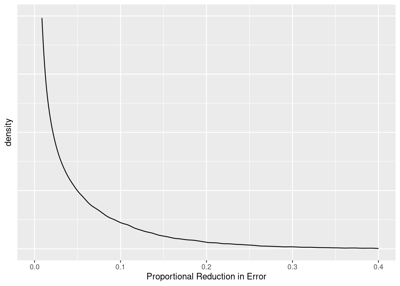
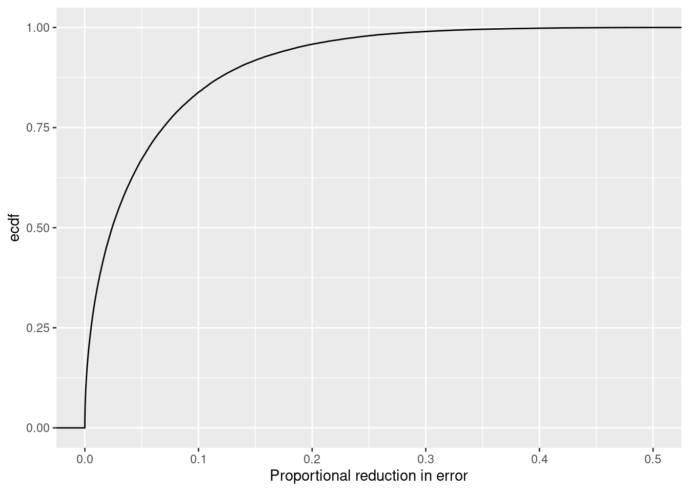
Now let’s plot the distribution of the PRE values we just generated:
So let’s return to the question of interest. The values of PRE observed in our original sample was 0.044. We wondered if this was sufficiently large to convince us to prefer the augmented model. We now know what values of PRE to expect when the compact model (i.e., the null hypothesis) is true. So we can compare our observed value of PRE to the distribution of PRE values under the null hypothesis to see whether our observed value of PRE is “large enough”. We can do so, but asking how often PRE takes on a value equal to or larger than our observed value of PRE. Mechanically, we can simply count how many of our 100000 samples (all of which were generated by the compact model) were equal to or larger than our observed value of PRE. It turns out, that 36220 of our 100000 samples (or 36.22%) are greater than or equal to 0.044.